Preface

How should students in climate science, meteorology, and physical oceanography learn mathematics? What topics in mathematics should they learn, and in what order? What changes are necessary in mathematics education for climate science students in order to meet the needs of climate science education and research in the big data era? In the last several decades, a typical undergraduate student enrolled in an atmospheric, oceanic, or climate science major might take six university-level mathematics and computing courses: Calculus I, II, and III, Linear Algebra and Differential Equations, Basic Statistics, and Computer Programming. This mathematics curriculum has several shortcomings, and two of them seem to us especially important: much of the mathematics that is taught has little relevance to a major such as climate science, and the pace of mathematics learning in this curriculum is too slow to meet the needs of the major courses. The textbooks used by climate science students in calculus, linear algebra, and statistics courses are usually written by mathematics and statistics professors, and much of the material in these books is simply not very relevant to practical climate science problems. The traditional approach to teaching mathematics treats calculus, linear algebra, statistics, differential equations, and computer programming as isolated and disconnected subjects. Consequently, this traditional teaching methodology not only makes these mathematics topics disconnected from each other, but also makes them even further disconnected from climate science. In reality, a typical climate science research problem does not present itself accompanied by a helpful statement as to what mathematical tools are needed to solve it. The tools can easily involve calculus, linear algebra, statistics, computer programming, or a combination of all these.

Therefore, climate science students have difficulty in seeing why mathematics is taught in this manner and in perceiving how mathematics is used in solving actual climate science problems. For example, a typical linear algebra course would never discuss the significance of eigenvalues in climate science and would never show how to compute the eigenvalues of a large climate data matrix. This pedagogical problem has puzzled many climate science educators for many years. Students are required to spend lots of time learning what they regard as irrelevant and peculiar topics in mathematics, such as using l’Hopital’s rule (named for the seventeenth-century French mathematician Guillaume de l’Hopital) to evaluate a limit, and a half-angle substitution to calculate an antiderivative, but these students then find themselves unable to cope with the mathematical demands of upper division and graduate-level climate science courses. As a result, climate science professors often complain about their students’ weak mathematics backgrounds, and the students in turn are frustrated with the inappropriate and abstract mathematical knowledge that they have acquired from mathematics professors who are unfamiliar with the climate science applications of mathematics. Conversely, the skills and techniques of data analysis and visualization, such as empirical orthogonal functions (EOFs), that are needed by virtually all climate science graduate students are simply not taught in the typical current sequence of mathematics classes that these students are required to take. In brief, conventional mathematics courses are not well suited to the mathematical needs of problems in climate science. Climate science students suffer from a serious mismatch between tasks and tools.

The question then arises as to how best to address the challenges and shortcomings of the current approach for climate science students to learn mathematics, an approach which is both disconnected and time-demanding. We have written this book to answer that question. Our book tries to overcome the above problems by blending the most climate-relevant materials of the six courses (Calculus I, II, and III, Linear Algebra and Differential Equations, Basic Statistics, and Computer Programming) with key climate science examples into one unified course, called Climate Mathematics. This single course may be taught in from one semester up to three semesters, depending on the qualifications and objectives of the students. Climate Mathematics presents the mathematical methods from the point of view of climate science applications. Climate Mathematics prepares climate science students with a sufficient mathematical background to enable them to take not only the upper division courses, but also most graduate-level climate science courses. It also prepares them to conduct research involving analysis and visualization of climate datasets.

Every important mathematical formula and each aspect of theory included in this book is presented together with at least one climate science example. At the same time, we have omitted many of the less relevant topics found in the typical array of six mathematics courses, such as limits in Calculus I, infinite series and integration techniques in Calculus II, determinants in Linear Algebra, and series solutions in differential equations. These omitted materials from the conventional mathematics curriculum are simply not used in typical current climate courses. Even if they are needed in some special cases, they can be more efficiently taught by the climate science instructor if his or her course needs them. We have also included some important modern topics that are not taught in the traditional six courses, such as the singular value decomposition (SVD) method to compute EOFs from a rectangular space–time data matrix.

The second defining feature of this book is the extensive use of computer codes. We have selected the programming language R for these codes. We provide an introduction to R for students to whom this remarkable language is completely new, and we include advanced R graphics suitable for application to global climate model (GCM) datasets. We also present R analysis and visualization techniques appropriate for observational climate datasets characterized by missing data.

The R codes are included in the book and are also available as an open source from the book website www.cambridge.org/climatemathematics. Also available from the book website are the equivalent computer codes written in Python. In recent years, Python has become a very popular computer language in science and engineering, and has begun to become popular among climate scientists. We have supplied a Python equivalent code for every R code in this book. The corresponding Python codes are available as an open source in the Jupyter Notebook format. They may be freely used by anyone.

The third distinct feature of the book is that we have also updated some topics based on recent advances in science and technology, such as the GPS-based radiosonde, a new hypsometric equation derived without the usual isothermal assumption, and the GPS-planimeter as a smartphone app to measure the area of a region on the Earth’s surface based on Green’s theorem.

We recognize that our book can be quite demanding for an instructor, who will ideally be familiar with all the mathematical tools we discuss, as well as the history of calculus, linear algebra, statistics, and computing. The instructor should also be conversant with the important applications of these tools to climate science, such as the SVD approach to EOFs and principal components, and techniques for the efficient analysis and visualization of Reanalysis GCM data. Perhaps at this moment not many instructors will be fully prepared to teach all the material in this book. However, this situation is changing rapidly. Currently, more Ph.D. students probably use SVD rather than a covariance matrix to compute EOFs. Many students are already skillful at employing data visualization and signal extraction using R, Python, and MATLAB packages. These graduate students can now use our book as a research reference and toolbox, and they will be well qualified to teach from our book when they become faculty members themselves. Thus, we in climate science and allied fields may learn from biology and psychology, which today are among the most popular majors in large public universities in the United States. Years ago, biology and psychology programs had begun to teach their own statistics courses, often staffed by biologists and psychologists. Engineering colleges had also started to teach their own linear algebra and differential equations courses. Calculus for Life Sciences and Calculus for Business are taught today on many campuses. We pose the following question: Should climate science departments or the geoscience college now begin to teach their own mathematics, statistics, and computing courses, using a book like this one, in the era of big data and artificial intelligence? Should climate science departments and mathematics departments make joint faculty appointments to teach Climate Mathematics? Or should the mathematics department first hire (if necessary) and then assign a faculty member who is thoroughly familiar with climate science to teach Climate Mathematics?

A closely related and important question is this: How should we teach the necessary mathematical methods to students who have decided to change their fields from humanities to climate science? These students typically come to climate science lacking a calculus background, and they may have no intention of employing the advanced mathematics needed for, say, climate modeling, but they can certainly contribute to interdisciplinary fields employing climate science, such as policy-making for climatic change. In fact, this book originated from lecture notes in a course created to teach exactly this type of student at Scripps Institution of Oceanography, University of California, San Diego. The course was called Climate Mathematics (SIOC 290). This course was taught by one of us (S.S.P.S.) and consisted of 45 hours of instruction in a special summer session of five weeks in 2015, with nine instruction hours per week. The course was designed for the students in a newly established program called Masters of Advanced Studies in Climate Sciences and Policy. These students would need to understand, explain, and present the results from climate models and observations. The students used SIOC 290 to prepare themselves to take graduate courses such as SIO 210 (Physical Oceanography), SIO 217A (Atmospheric Thermodynamics), and SIO 260 (Marine Chemistry). In addition to strictly mathematical topics, the students taking this course would also learn sufficient graphics and visualization techniques to enable them to present and describe climate data from both observations and models. SIOC 290 was taught again in 2016 and a third time in 2017.

In choosing the title Climate Mathematics, we wished to emphasize that this book is not aimed at a mathematics class for mathematics majors. Several in-depth mathematics courses on the topics we cover, such as linear algebra, can and should be taught for mathematics majors and other students who love mathematics for its own sake. Also, in order to limit this book to a reasonable size, we have not included several aspects of mathematics that are useful in climate science. Numerical methods for ordinary and partial differential equations, for example, are essential for climate modeling, but they are beyond the scope of this book. We hope to include them in a future book on Advanced Climate Mathematics.

Suggestions on the Usage of the Book

Who Will Use this Book?

This book can be used as both a textbook and a reference manual for the following five groups of students as illustrated in Fig. 0.1.

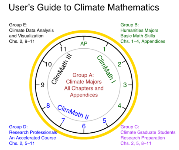
Figure 0.1. Schematic diagram illustrating how this book might be used in several different courses for students having different backgrounds and motivations. ClimMath I, II, and III stand for three semesters of Climate Mathematics course based on this book. ClimMath I covers the basics of Calculus in the Appendices (denoted by AP in the 12 o’clock position), R Program in Chapter 2, Statistics in Chapter 3, and Linear Algebra in Chapter 4. ClimMath II covers Chapters 5–8 and focuses on the methods of climate modeling as applications of the mathematical methods described in ClimMath I. ClimMath III covers Chapters 9–11 plus one or two research topics selected by an instructor, and focuses on climate data analysis and visualization.
Group A. This group includes undergraduate students majoring in climate science, meteorology, or oceanography. The book can be used as a textbook for three semesters of Climate Mathematics I (Appendices, Chapters 1–4), II (Chapters 5–8), and III (Chapters 9–11) to replace the traditional six semesters of courses: Calculus I, II,and III, Linear Algebra and Differential Equations, Basic Statistics, and Computer Programming. Climate Mathematics I contains an accelerated introduction to calculus including the divergence theorem and line integrals, and it prepares students to take courses in mechanics and atmospheric or oceanic dynamics and thermodynamics. When students complete all the three Climate Mathematics courses, they should have sufficient quantitative analysis background to take upper division undergraduate courses in climate science, such as the courses based on the book by Wallace and Hobbs entitled Atmospheric Science: An Introductory Survey, that by Talley et al. entitled Descriptive Physical Oceanography: An Introduction, and that by Curry and Webster entitled Thermodynamics of Atmospheres and Oceans. Students should have also mastered sufficient skills for data analysis and data mappings for course work and research projects. Because students complete the mathematics training early in their undergraduate programs,they will have more time to take newly created courses, such as machine learning in climate science, geographic information systems (GIS), satellite meteorology,climate data visualization, or climate modeling.Alternatively, a student might choose to accelerate the Climate Mathematics series by taking Climate Mathematics II and III simultaneously in the second semester of the freshman year. This would allow the student to have more freedom to choose her/his courses, particularly the big data courses that will dramatically improve the employment opportunities of the climate science majors.

Group B. This group includes those students who originally were humanities majors, but now wish to change their emphasis to climate science or simply to take several upper division or graduate climate science courses. They had not majored in physical sciences and have little background in calculus, statistics, or linear algebra, but they are well motivated to learn climate science. Yet they have no time to go through the full series of Climate Mathematics I, II, and III. They prefer to have the minimum mathematics background necessary to enable them to take a few upper division climate science courses. The background can be achieved by taking one semester simplified Climate Mathematics using selected sections from our book as the text. We suggest the following sections: Appendices A, B, C, and D.1, D.3, D.4.1–2, D.4.5–7, and Chapters 1.1–1.4, 2.1–2, 3.1–3, 5.1–2, 6.4–7, and 7.1–2. This course may be called Climate Mathematics B.

Group C. This group includes the graduate students in climate science who have received the traditional mathematics education and wish to enhance or refresh their modern mathematical skills for research, such as the energy balance models, modern hypsometric equation, R analysis of the GCM data, and data visualization. This can be a one-semester course, called Climate Mathematics C, which uses Chapters 2 and 5, Section 7.2, and Chapters 8–11. It is basically Climate Mathematics III plus some selected topics to prepare for climate science research. Because the students have already taken at least the six traditional mathematics courses, Climate Mathematics C can be taught at an accelerated pace compared to Climate Mathematics III.

Group D. This group includes research scientists and professionals who wish to modernize their skills in modern mathematics, statistics, climate data analysis, and data visualization. They may take a one-semester selected topics course with the topics selected from Chapters 2 and 5–11. This is Climate Mathematics D.

Group E. This group includes people who are mainly interested in climate data analysis and visualization, such as climate science professionals in government laboratories or businesses. They might spend a week-long effort with this book in preparation for working on R analyses and graphics for climate data. They can study topics from Chapters 2 and 9–11 to learn how to analyze and visualize climate data for presentations or research, such as R plotting for climate data and a comprehensive R analysis for the gridded United States surface temperature data. One of us (S.S.P.S.) taught such a short course in 2017 for scientists at the National Centers for Environmental Information in the United States, and also at the Chinese Academy of Sciences in Beijing.
Because this book contains numerous R codes for climate data analysis and graphics,the book can also be used as a reference manual for a climate scientist. The book’s website www.cambridge.org/climatemathematics provides updated computer codes in both R and Python to support all users of this book.

How to Use this Book
We have tried to make this book “user-friendly” for both students and instructors. An instructor can simply follow the book when lecturing and can assign the exercise problems. Complete solutions for a few selected problems are presented at the end of the book as Appendix E to help train students in writing about mathematics. A solutions manual with answers for all the problems is available through the publisher to qualified instructors.

This book emphasizes the value of practice in acquiring quantitative analysis skills.The book contains many R codes, which can also be found at the book’s website www.cambridge.org/climatemathematics showing details of our R codes and their output. The relevant climate data used in the R codes can also be downloaded directly from the website.

The exercise problems that require R codes are marked with a computer symbol.Problems that do not have this symbol can be solved analytically without using a computer.

When doing computations, we strongly recommend that readers of conventionally published books should use the R codes (or their Python equivalents) that can be found on the book’s website, www.cambridge.org/climatemathematics. There is no need to retype the computer codes. The open-source online codes will be maintained and will include corrections, updates, and improvements to the original codes. Although e-book readers may be able to copy and paste the R code from a pdf file to RStudio, some special symbols, such as ~  and ^ , may become altered in this copy-and-paste procedure and may have to be corrected in RStudio.

The websites cited in this book may be updated or changed in the future. Readers can find the updated website addresses on the book website www.cambridge.org/climatemathematics.

The datasets used in this book can be downloaded as a data.zip file from the book website: www.cambridge.org/climatemathematics. Updated data in some cases can be downloaded from the data developers’ websites provided in the book.

A new mathematics textbook of this size is virtually certain to contain errors, despite the diligent efforts of many people to find them all before publication. We take full responsibility for all remaining errors, and we will post any errata on the book’s website,www.cambridge.org/climatemathematics.